Graph Neural Networks are everywhere. They power the recommendation engines that suggest your next purchase, detect fraudulent transactions in real-time, and recently, they’ve become crucial infrastructure for Retrieval-Augmented Generation (RAG) systems that help Large Language Models access external knowledge. GNNs consistently outperform simpler alternatives on graph-structured data.

But here’s the uncomfortable truth: when it comes to deploying these models in production, industry often chooses not to use them.

The reason? Latency. GNNs are computationally expensive. Every time you want to make a prediction, the model needs to recursively aggregate information from neighbors through multiple layers of message passing. In a social network with millions of users or a knowledge graph with billions of entities, this means fetching data across the network, aggregating features from potentially thousands of neighbors, and propagating information through several layers — all before you can make a single prediction.

This creates what we call the performance-efficiency dilemma: GNNs offer high accuracy but slow, resource-heavy inference. Multi-Layer Perceptrons (MLPs) are incredibly fast — just straightforward matrix multiplications, no graph operations, no neighbor lookups — but they’re structurally blind. They treat each node in isolation, ignoring all the rich relational information that makes graphs useful in the first place.

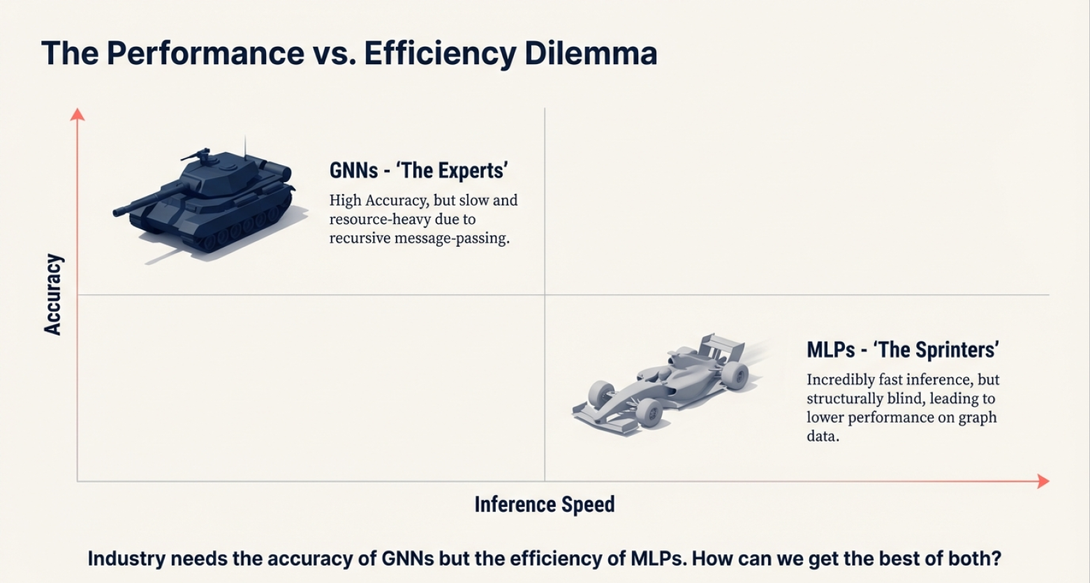
The performance gap is substantial. On the Cora citation network, a vanilla MLP achieves around 58% accuracy, while a GCN reaches about 82%. That’s not a gap you can easily ignore [1].

So the question becomes: can we get the best of both worlds? Can we build a model that’s as fast as an MLP at inference time, but captures the structural knowledge of a GNN?

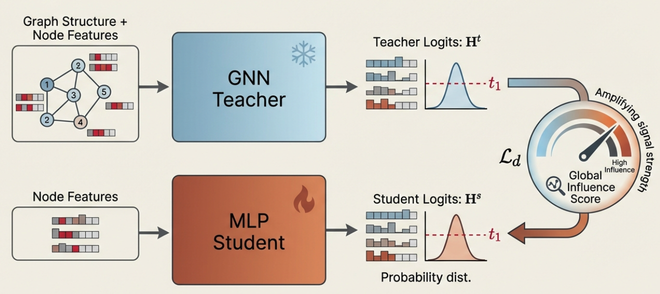
This is where knowledge distillation enters the picture. The idea is elegant: train a powerful GNN teacher on the graph, then transfer its knowledge to a lightweight MLP student. At deployment time, you throw away the expensive teacher and deploy only the fast student. The student inherits structural understanding without needing to perform message passing.

This approach, pioneered by GLNN (Graph-Less Neural Networks)[2], shows real promise. Distilled MLPs can close much of the performance gap with their GNN teachers while maintaining inference speeds that make them practical for production deployment.

But here’s where it gets interesting: how exactly should we transfer this knowledge?

Most existing methods treat all nodes in the graph equally during distillation. They assume every node contributes the same amount to the training loss. Some recent work recognized this might be suboptimal and introduced non-uniform approaches. Methods like KRD [3] and HGMD [6] use prediction entropy to discriminate between nodes: nodes where the teacher is less confident get more attention during training.

The reasoning seems sound: uncertain predictions are “harder” samples, so we should focus on them.

But think about this for a moment. Entropy measures how confident the teacher GNN is about a node’s label. It doesn’t tell you anything about the node’s role in the graph structure. A node could have high entropy simply because its features are ambiguous, not because it’s structurally important.

This led us to ask a different question: “How influential is this node within the structure of the graph?”

In this post, I’ll walk you through InfGraND, our influence-guided approach to GNN-to-MLP knowledge distillation that was recently published in Transactions on Machine Learning Research (TMLR). We’ll cover the intuition, the key ideas, and why asking about structural influence leads to better results than asking about prediction confidence.

The Pebble in the Pond #

Here’s an intuition that helped us think about node influence:

Imagine dropping pebbles into a pond. Some pebbles create ripples that spread far across the water; others barely disturb the surface. The size and reach of the ripples depend on where you drop the pebble and how the water flows.

Graphs work similarly. When you perturb a node’s features, that perturbation propagates through message passing to affect other nodes’ representations. Some nodes, by virtue of their position in the graph, have perturbations that ripple far and wide. Others have more localized effects.

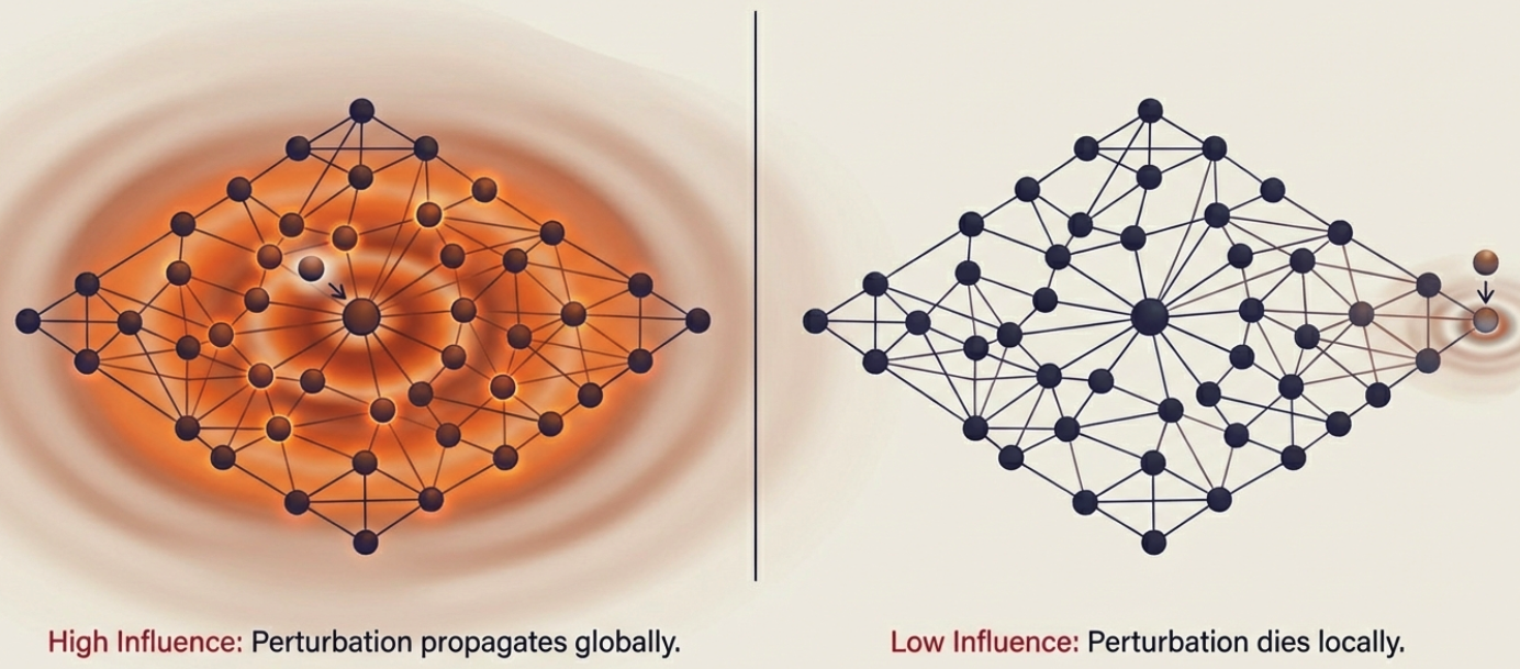
We call this “influence” and it’s fundamentally a structural property.

Measuring Node Influence #

How do we actually quantify this? Formally, we define the influence of a source node $v_i$ on a target node $v_j$ after $k$ message-passing iterations as:

$$\hat{I}_{(j \leftarrow i)}(v_j, v_i, k) = \left| \mathbb{E}\left[\frac{\partial \mathbf{x}_j^{(k)}}{\partial \mathbf{x}_i^{(0)}}\right] \right|_1$$

In plain terms: we’re measuring how much the target node’s representation changes when we perturb the source node’s initial features. The Jacobian captures this sensitivity, and the L1-norm gives us a scalar measure.

Computing this exactly is expensive, but we can approximate it efficiently. Following the insight from Simplified Graph Convolutional Networks (SGC) [7], we remove non-linearities and weight matrices to focus on pure topological propagation:

$$\mathbf{X}^{(k)} = \tilde{\mathbf{A}}\mathbf{X}^{(k-1)}$$

where $\tilde{\mathbf{A}}$ is the normalized adjacency matrix. After $k$ propagation steps, we use cosine similarity between the original features $\mathbf{x}_i^{(0)}$ and the propagated features $\mathbf{x}_j^{(k)}$ as our influence indicator.

The beauty of this approach? It’s parameter-free and computed only once as a preprocessing step — no overhead during training or inference.

To get a single importance score per node, we aggregate pairwise influences into a Global Influence Score:

$$I_g(v_i) = \frac{\sum_{j \in V} I_{(j \leftarrow i)}(v_j, v_i, k)}{\max_{l \in V} \sum_{j \in V} I_{(j \leftarrow l)}(v_j, v_l, k)}$$

This tells us how much each node influences the entire graph, normalized to lie between 0 and 1.

Does Influence Actually Matter? #

Before building a whole framework around influence, we wanted to verify our hypothesis: does training on high-influence nodes actually lead to better models?

We ran a simple experiment. For each dataset, we split the training nodes into two groups: the top 25% by influence score (high-influence) and the bottom 25% (low-influence). Then we trained separate GNNs on each subset using the same test set.

The results were consistent across all datasets and GNN architectures: models trained on high-influence nodes significantly outperformed those trained on low-influence nodes. This validated our core intuition — influence captures something meaningful about which nodes matter most for learning.

InfGraND: Putting It All Together #

With influence validated as a useful signal, we built InfGraND (Influence-Guided Graph Knowledge Distillation) around two main components:

1. Influence-Guided Distillation Loss #

Instead of treating all nodes equally, we weight the distillation loss by influence scores. For each node $i$, we encourage its representation to match the teacher’s predictions for its neighbors $j$, weighted by how influential those neighbors are:

$$\mathcal{L_d} = \sum_{i \in V} \sum_{j \in \mathcal{N}(v_i)} w_{ij} \cdot \text{KL}(p_i^s, p_j^t)$$

where $p_i^s = \sigma(\mathbf{h}_i^s / \tau)$ and $p_j^t = \sigma(\mathbf{h}_j^t / \tau)$ are the student and teacher probability distributions, and the weight for each neighbor is:

$$w_{ij} = (\gamma_1 + \gamma_2 \cdot I_g(v_j)) \cdot \frac{1}{|\mathcal{N}(v_i)|}$$

Let’s break this down:

• $\gamma_1$ provides a baseline gradient from all neighbors (we don’t completely ignore low-influence nodes)
• $\gamma_2 \cdot I_g(v_j)$ amplifies the signal from high-influence neighbors
• $D_{KL}$ is the KL divergence between student and teacher predictions
• $\tau$ is the distillation temperature

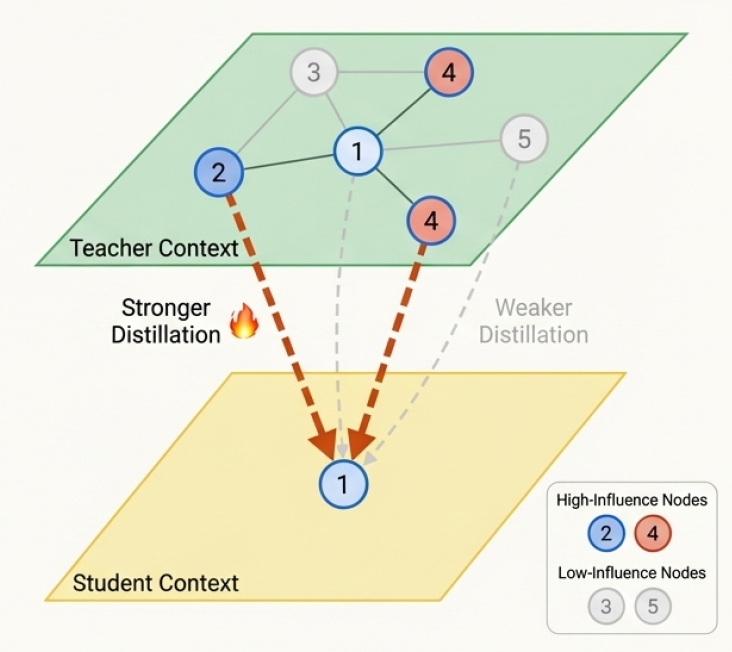
The key insight: high-influence neighbors provide stronger supervision signals. The student learns to prioritize getting these nodes right.

2. One-Time Feature Propagation #

To give the MLP some structural awareness without adding inference overhead, we pre-compute multi-hop neighborhood features:

$$\tilde{\mathbf{X}} = \text{POOL}\left({\mathbf{X}^{(p)}}_{p=0}^{P}\right)$$

We propagate features through the graph structure for $P$ hops, then average-pool across hops. This enriched feature matrix $\tilde{\mathbf{X}}$ becomes the input to our MLP.

The critical point: this is computed once before training and stored. At inference time, the MLP just uses these pre-computed features — no graph operations needed.

The Complete Objective #

The student MLP is trained with a combination of supervised loss (on labeled nodes) and distillation loss (on all nodes):

$$\mathcal{L}_t = \lambda \mathcal{L}_s + (1 - \lambda) \mathcal{L}_d$$

Both losses incorporate influence weighting, ensuring that structurally important nodes guide both the ground-truth learning and the knowledge transfer from the teacher.

Results: Does It Work? #

We evaluated InfGraND across seven benchmark datasets in both transductive and inductive settings, comparing it against state-of-the-art baselines including GLNN, KRD (entropy-based distillation), and HGMD.

The results tell a compelling story.

Influence beats confidence. Across all datasets and teacher architectures (GCN, GAT, GraphSAGE), our influence-guided approach consistently outperformed entropy-based methods that rely on prediction confidence. This validates our core hypothesis: asking “how structurally important is this node?” is more effective than asking “how uncertain is the teacher?”

Students can surpass their teachers. Perhaps the most surprising finding: the distilled MLP student frequently achieved higher accuracy than its GNN teacher. The distillation process itself, when guided by influence, acts as a form of beneficial regularization that helps the student generalize better than the teacher.

Speed AND accuracy. InfGraND doesn’t just match GNN performance while being faster, it actually exceeds GNN accuracy while being 6-14x faster at inference time. This breaks the typical speed-accuracy tradeoff. You get both better results and dramatically lower latency, making deployment in production environments genuinely practical.

Massive gains over vanilla MLPs. Compared to MLPs trained without any distillation, InfGraND delivered double-digit percentage improvements in accuracy, effectively closing the gap between blind MLPs and structure-aware GNNs.

Both components matter. Our ablation studies showed that both the influence-guided loss and the one-time feature propagation contribute meaningfully to performance. Removing either component degrades results, but they’re complementary—together, they create something greater than the sum of parts. The influence weighting helps the model learn from the right nodes, while feature propagation provides structural context.

Works even with limited labels. In label-scarce scenarios (using only 10-40% of training labels), InfGraND maintained its advantage over baselines. When supervision is limited, influence-guided distillation becomes even more valuable by helping the model focus on the most informative examples.

For detailed experimental results, complete benchmarks, statistical significance tests, and comprehensive ablation studies, please refer to our full paper.

What We Learned #

A few takeaways from this work:

The right question matters. Shifting from “how confident is the teacher?” to “how influential is this node?” led to consistent improvements. Sometimes reframing the problem is more valuable than building more complex solutions.

Structure can be baked in without runtime cost. The one-time feature propagation gives MLPs structural awareness at zero inference cost. This is inspired by industrial practices like embedding lookup tables — precompute what you can.

Simpler students can outperform complex teachers. With the right training signal, MLPs can exceed GNN performance while being much faster. This has real implications for deploying graph-based models in production.

Try It Yourself #

The code is available on GitHub: https://github.com/AmEskandari/InfGraND

The paper is published in TMLR and available on OpenReview: https://openreview.net/forum?id=lfzHR3YwlD

If you’re working on graph-based applications where inference speed matters, give InfGraND a try. And if you have questions or ideas for extensions, feel free to reach out.

References #

[1] Eskandari, A., Anand, A., Rashno, E., & Zulkernine, F. (2026). InfGraND: An Influence-Guided GNN-to-MLP Knowledge Distillation. Transactions on Machine Learning Research.

[2] Zhang, S., Liu, Y., Sun, Y., & Shah, N. (2022). Graph-less Neural Networks: Teaching Old MLPs New Tricks via Distillation. ICLR.

[3] Wu, L., Lin, H., Huang, Y., & Li, S. Z. (2023). Quantifying the Knowledge in GNNs for Reliable Distillation into MLPs. ICML.

[4] Kipf, T. N., & Welling, M. (2016). Semi-Supervised Classification with Graph Convolutional Networks. ICLR.

[5] Hamilton, W., Ying, Z., & Leskovec, J. (2017). Inductive Representation Learning on Large Graphs. NeurIPS.

[6] Wu, L., et al. (2024). Teach Harder, Learn Poorer: Rethinking Hard Sample Distillation for GNN-to-MLP Knowledge Distillation.

[7] Wu, F., Souza, A., Zhang, T., Fifty, C., Yu, T., & Weinberger, K. (2019, May). Simplifying graph convolutional networks. In International conference on machine learning.

Bibtex #

@article{eskandari2026infgrand,
  title={InfGraND: An Influence-Guided GNN-to-MLP Knowledge Distillation},
  author={Eskandari, Amir and Anand, Aman and Rashno, Elyas and Zulkernine, Farhana},
  journal={Transactions on Machine Learning Research},
  year={2026},
  url={https://openreview.net/forum?id=lfzHR3YwlD}
}